The easy way to create an array of numbers is to get a bunch of zeros or ones using convenient functions.

np.zeros(shape=(n_rows,n_cols))
np.ones(shape=(n_rows,n_cols))

While this works for some cases, in many others we want the elements of the array to be diverse rather than repeating. At this point hardly anyone thinks about creating a magic square! They do satisfy the diversity criteria, but numpy natively does not have methods to create magic squares. So we will skip them! The popular choice is random numbers. Numpy has a whole bunch of methods to create random numbers. https://docs.scipy.org/doc/numpy-1.13.0/reference/routines.random.html lists all the methods numpy.random has and they are sufficient for almost all our needs. Numpy has a good collection of simple methods for generating random numbers - rand, random, ranf, randn etc. The problem with these is the non intuitive names and the overlap of features provided by these functions.

Here are the confusions introduced be these functions:

• When you have a tuple/list for size everywhere in numpy, why not for rand?

  rand(d0, d1, ..., dn) #Random values in a given shape.
  

• Can’t randn be named as rand_normal?

  randn(d0, d1, ..., dn) #Return a sample (or samples) from the “standard normal” distribution
  

• random, randf and sample provide the same functionality as random_sample

  random_sample([size]) #Return random floats in the half-open interval [0.0, 1.0)
  random([size]) #Return random floats in the half-open interval [0.0, 1.0)
  ranf([size]) #Return random floats in the half-open interval [0.0, 1.0)
  sample([size]) #Return random floats in the half-open interval [0.0, 1.0)
  

The functions for distributions do not suffer from this problem. But they are less frequently used. Almost every code you see that needs a random number has np.random.rand() or np.random.random(). They do the same thing - pick numbers in [0.0,1.0) uniformly. So does np.random.ranf().

np.random.seed(100); np.random.rand(7)
# array([ 0.54340494,  0.27836939,  0.42451759,  0.84477613,  0.00471886, 0.12156912,  0.67074908])
np.random.seed(100); np.random.random(7)
# array([ 0.54340494,  0.27836939,  0.42451759,  0.84477613,  0.00471886, 0.12156912,  0.67074908])
np.random.seed(100); np.random.ranf(7)
# array([ 0.54340494,  0.27836939,  0.42451759,  0.84477613,  0.00471886, 0.12156912,  0.67074908])

Would it not be easier to use np.random.uniform(size=(7)) instead? Though it has little more typing to do, it is easier to understand and explicitly tells how the random number is generated. To generate numbers in a range other than [0.0, 1.0)- say [2,5)- using rand or random methods you would have to resort to (5-2)*np.random.random()+2. Using uniform you can achieve it as np.random.uniform(2,5,7). It is better to forgo the convenient, obscure simple random number functions and use the actual distribution functions themselves.

The 80-20 rule (Pareto Principle) in action

Remember the 80-20 rule? It says that approximately 80% of the results come from just 20% of the total effort, i.e. a few actions provide disproportionate gains. It does apply here. Three easy distribution functions in numpy will cover the majority of your random number needs.

The Pareto principle (also known as the 80/20 rule, the law of the vital few, or the principle of factor sparsity) states that, for many events, roughly 80% of the effects come from 20% of the causes

The most common distributions we encounter are uniform or normal distributions.

1. Uniform distribution

   Uniform distribution captures the idea that all are equal - every number in a given range have the same chance (probability) of appearing in the result

   np.random(low=0.0, high=1.0, size=None)
   # range in which the random number need to fall is [low, high)
   

   Some examples:

   • 5 uniformly distributed numbers in range [0.0,1.0) (i.e. emulating functionality of rand or random or ranf methods)

       np.random.uniform(size=5)
     

   • 2x3 uniformly distributed numbers in the range [a, b)

     np.random.uniform(a, b, (2,3))
     #np.random.uniform(low=a, high=b, size=(2,3))
     

   • 2x3 uniformly distributed integers numbers in the range [a, b)

     np.random.uniform(a, b, (2,3)).astype(np.int32)
     #np.random.uniform(low=a, high=b, size=(2,3)).astype(np.int32)
     

2. Normal distribution (Bell Curve/Gaussian Distribution)

   Normal distribution enables a way of picking numbers (mostly) from a bell shaped region. The shape of the bell is determined by the standard deviation (which directly controls the width of the bell shape and inversely controls the height of the bell). The position of the center of the base of the bell is determined by the mean. This is a simplistic definition to aid visualization of the curve.

   

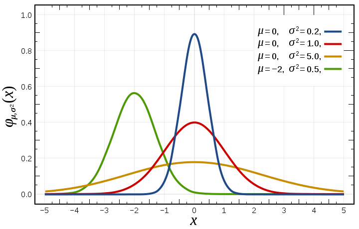
   Normal distribution with mean=0 and standard deviation=1 is called Standard Normal distribution.

   p.random.normal(loc=mean, scale=standard_deviation, size=None)
   #loc and scale specify the mean and standard deviation values used to describe a normal distribution
   

   Some examples:

   • 5 standard normal distributed numbers

       np.random.normal(size=5)
     

   • 2x3 numbers from the normal distribution with mean=70, and standard deviation=4

     np.random.normal(70,4,(2,3))
     #np.random.normal(loc=70, scale=4, size=(2,3))
     

   • 2x3 integers from the normal distribution with mean=70, and standard deviation=4

     np.random.normal(70,4,(2,3))astype(np.int32)
     #np.random.normal(loc=70, scale=4, size=(2,3))astype(np.int32)
     

3. Binomial Distribution

   If we toss a fair coin many many times, we get equal number of heads and tails. What if the coin is not fair and tends to land on one side more than other, the final outcome is biased to the side that has a higher chance. The results in these two situations follow the binomial distribution.

   In probability theory and statistics, the binomial distribution with parameters n and p is the discrete probability distribution of the number of successes in a sequence of n independent experiments, each asking a yes–no question, and each with its own boolean-valued outcome: a random variable containing single bit of information: success/yes/true/one (with probability p) or failure/no/false/zero (with probability q = 1 − p). A single success/failure experiment is also called a Bernoulli trial or Bernoulli experiment and a sequence of outcomes is called a Bernoulli process; for a single trial, i.e., n = 1, the binomial distribution is a Bernoulli distribution.

   np.random.binomial(n=number_of_tosses, p=probability_of_landing_on_head, size=None)
   

   Some examples:

   • Toss a fair coin 20 times and repeat this experiment 5 times

       np.random.binomial(20, 0.5, size=5)
       #np.random.binomial(n=20, p=0.5, size=5)
     

   • 2x3 numbers from a binomial distribution after 1000 trails(tosses) and probability of success is 0.8

     np.random.binomial(1000, 0.8, size=(2,3))
     #np.random.binomial(n=1000, p=0.8, size=(2,3))
     

As the Pareto principle goes, these three distributions should take care of the majority of your random number needs.

It is easy to remember these three functions. I call these the BUN functions - Binomial, Unifrom and Normal. All the three have size as the common, optional, third argument which if not mentioned returns a single value. The first two arguments to each of these functions are the parameters for generating the distribution.

BUN(?, ?, size)

These have sensible defaults for the first and second arguments if nothing is specified:

• low=0.0 and high=1.0 for the uniform distribution (which explains np.random.uniform())
• loc(mean)=0.0 and scale(std)=1.0 for normal distributions which is a standard normal distribution (which also explains the result of np.random.normal())
• binomal needs the first two arguments to be specified as they no defaults though one could argue that n=100 and p=0.5 (100 tosses of a fair coin) could make decent defaults.