Matrix Multiplication - A different perspective
Matrix multiplication is a common operation we come across in engineering and mathematics. We see it a lot in machine learning algorithms. Unlike multiplication of scalars we have a prerequisite for matrices (i.e. number of columns in first matrix = number of rows in second matrix). The output of a valid matrix multiplication has output rows=number of rows in first matrix and output columns=number of columns in second matrix. I visualize matrix multiplication in a XY-grid for validating the feasibility of multiplication and to determine the shape of the output matrix. We will explore in this method in this article.
The idea is to arrange both the matrices in two of the XY-grid quadrants, and use a visual property in the other two quadrants to validate, and determine the shape of the output matrix.
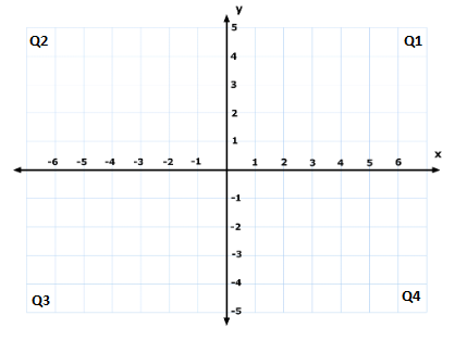
First some conventions: Of the four quadrants in XY-grid, Q1 is top-right, Q2 is top-left, Q3 is bottom-left and Q4 is bottom-right, as shown below.
Now lets say we have to multiply matrices A and B. A has shape 2x3 and B is a 3x4 matrix. Below are the steps to setup the matrices in the grid and interpret the result.
- Fit the first matrix, A in the corner of Q3 (at the origin).
- Similarly, fit the second matrix B in the corner of Q1 (at the origin).
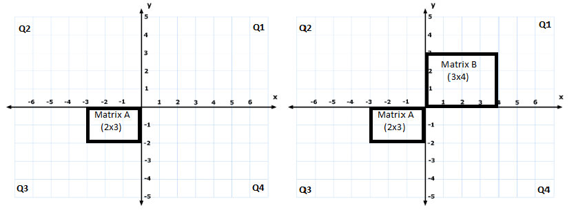
Matrix A in Q3 and matrix B in Q1 - Now some visuals:
Imagine shafts of light originating from each of the four edges of these two matrices.
It will be like below for Matrix A and B: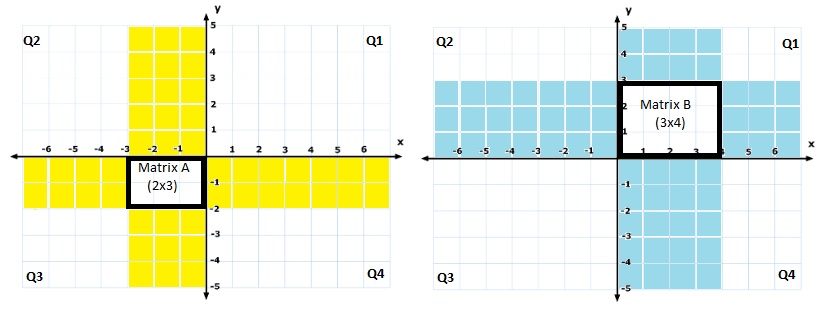
Matrix A shafts, Matrix B shafts - Light shafts from these two matrices overlap at two places, in Q2 and Q4.
The overlapping sections are the rectangles in green (blue+yellow=green).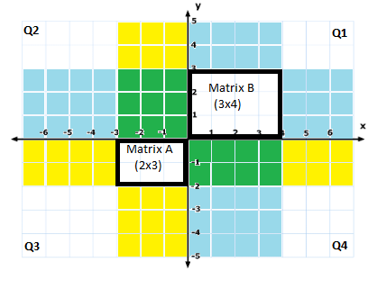
We have a green 3x3square in Q2 and a green2x4rectangle in Q4 - Our setup is done. Examining Q2 and Q4 we can determine if these two matrices can be multiplied, and if so, the shape of the output matrix.
Look at Q2. If the overlap region (shown in green below) is a square then these matrices can be multiplied. Else not. - If above check fails we know these matrices cannot be multiplied. If check succeeds, (i.e. multiplication is feasible) then look at the green overlap region in Q4. The shape of the overlap region is the shape of the output matrix. That’s it!
Examples
Lets walk through a few examples to make it concrete. For the following three examples we calculate A * B.
- Let A be a
3x1matrix (a column vector) and B be a1x3matrix (a row vector). Putting A in Q3, and B in Q1 we examine Q2. The overlap in Q2 is a square (1x1). So we can multiply A and B. And the output is a3x3matrix (green overlap region in Q4). This is called outer product.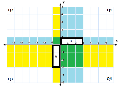
Vector Outer Product - Now, let A be a
1x4matrix (row vector) and B a4x1matrix (column vector). The overlap in Q2 is a4x4square region. So multiplication is possible. The output (overlap size in Q4), is a 1x1 matrix. In other words, the output is a scalar. This matrix multiplication is the popular vector dot product/dot product.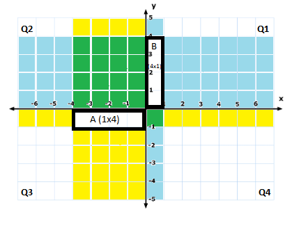
Vector Dot Product - Now lets try multiplying incompatible matrices. Let A be a
4x2matrix and B a4x5matrix. In this case, the overlap region in Q2 is not a square (but a4x2rectangle). So, these matrices cannot be multiplied.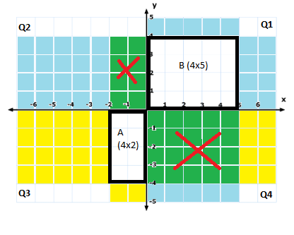
Invalid Matrix Multiplication
Note
If we need to do B * A instead of A * B, we normally would shift A to Q1 and B to Q3 and repeat the process. But, we can do that without changing the position of A and B - validate in Q4 and get output shape in Q2. Look for a square in Q4. If so, then overlap in Q2 has the output shape of B * A.
So, keeping A and B fixed in Q1 and Q3 respectively, we can visualize both A * B and B * A.
If the placement of A and B in Q1 and Q3 is uncomfortable for you, you can change it.
In general, we place A and B in any diagonal quadrants (i.e. in the odd or even quadrants). We need to examine the other diagonal quadrant for validation and output shape. The quadrant horizontal to the second matrix should have a square overlap and the quadrant horizontal to the first matrix has the output shape. For A * B, A is the first and B is the second matrix. For B * A, B is the first and A is the second matrix.
For instance, if we place A in Q2 and B in Q4 and want to compute B * A, validation (square overlap) happens in Q1 (horizontal to Q2 where we have the second matrix, A) and output shape is visible in Q3 (horizontal to Q4 where we have the first matrix, B).
Back to the basics
All this time it was assumed you knew how to multiply two matrices. Well if you don’t know, here is how.

3x3 square in Q2 and a green 2x4 rectangle in Q4The figure above is the multiplication of A and B. We know that the output shape is 2x4. Lets call each of the 8 (2*4=8) small green (1x1) squares in Q4 a cell. Each cell in Q4 is the result of a vector dot product of a row vector and column vector (similar to Example 2). The value of cell at 1st row, 2nd column of Q4 is the vector dot product of 1st row of A (which is a row vector) and 2nd column of B (which is a column vector). The value of cell at 2nd row, 4th column of Q4 is the vector dot product of 2nd row of A (a row vector) and 4th column of B (a column vector), as shown in figure below. In general, value of every cell in the output is the dot product of the corresponding row in A and corresponding column in B.
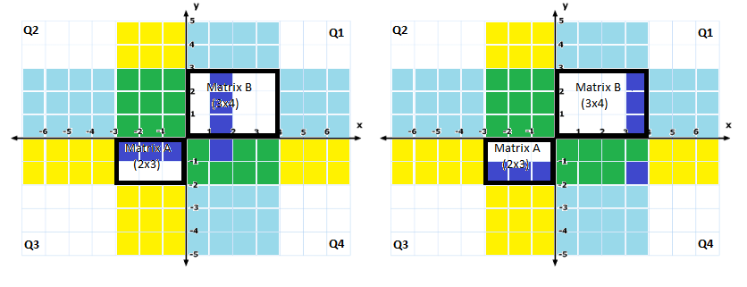
If we do this systematically, the first row of the output matrix is computed by the dot product of first row of A with each of the columns of B. Do the same for the second row of output matrix same as above, but using the second row of A instead of the first row. Repeat this till the the last row of A. Now you have multiplied matrices A and B.
Matrix multiplication can be interpreted as the (vector) dot product of every row in the first matrix with every column in in the second matrix.
As a fun exercise you can infer some properties of matrix multiplication using this representation.